To build our simulation, we'll first need to find discrete solutions for Keplerian potential. The core of Keplerian potential is a two body system, with one body orbiting the other. Assuming no other forces interact with these bodies besides gravity, the stable orbit has an eccentricity of 0¹, which is a circle. We'll define this with a few constants:

#CONSTANTS
GM = 6.673e-8*2.e33 #gravitational constant * solar mass
au = 1.495e13 #astronomical unit
year = 3.1557e7 #tropical year (see https://en.wikipedia.org/wiki/Tropical_year)
kms = 1.0e5 #km/s
ecc = 0 #eccentricty of orbit
tmax = 10.*year #maximum time
nsteps = 100 #number of steps to take
dt = tmax/nsteps #change in time per step (take smaller steps for more data and visa versa)
an = [0, 0] #acceleration

Next, we need to plot the circle with a radius of 1 AU around the center of the graph, so we'll write a function to generate a basic circular orbit and plot it onto a 2D plane.

def stableOrbit(r, phi):
    return r*np.cos(phi), r*np.sin(phi)

def plotStbOrbit(timesteps):
    phis = np.linspace(0, np.pi*2, timesteps/(tmax/year))
    stableX = []
    stableY = []
    for i in range (0, int(tmax/year)):
        sX, sY = stableOrbit(1*au, phis)
        stableX = np.append(stableX, sX)
        stableY = np.append(stableY, sY)
    stableX = stableX[:len(stableX)-1]
    stableY = stableY[:len(stableY)-1]
    return stableX, stableY

To evolve a simulation, we'll need to define a timestep, which is how much the simulations evolves at once. We'll use 1000 as the timestep, which translates to 1000 steps over the course of 10 years.

We've built the basic stable simulation, set up constants, so now we're ready to begin modeling. Using something called Euler methods, first described by Leonhard Euler, who solved these ordinary differential equations using Taylor expansions. There's two types of Euler methods, forward and modified Euler methods. We'll take it slow and start with the equations for the Forward Euler method:

\(\begin{gathered} (v^{n+1}_p = v^{n}_p + a(x^{n}_p)\Delta t) \end{gathered}\)

\(\begin{gathered} (x^{n+1}_p = x^{n}_p + v^{n}_p\Delta t) \end{gathered}\)

with \((x)\) as the dimension, \(v\) as the velocity, and \(\Delta t\) as the change in a single timestep. The first equation states that the velocity for the next timestep is equal to the velocity of the current timestep plus the product of the acceleration, current space, and the change in a timestep. This is just a reordering of the equation that acceleration is simply the difference between velocities. The second equation is just as simple, telling you that the next position will be the sum of the current position and the product of the velocity and time. The faster something moves, the further away it'll be at the next timestep. How did we get these equations? The full Taylor series expansion is:

\(\begin{gathered} x^{n+1}_p = x^{n}_p + \dot x^{n}_p \Delta t + 1/2 \ddot x^{n}_p \Delta t^{2} + \mathcal{O}(\Delta t^{3}) \end{gathered}\)

\(\begin{gathered} = x^{n}_p + v^{n}_p \Delta t + \mathcal{O}(\Delta t^{2}) \end{gathered}\)

\(\begin{gathered} v^{n+1}_p= v^{n}_p + \dot v^{n}_p \Delta t + 1/2 \ddot v^{n}_p \Delta t^{2} + \mathcal{O}(\Delta t^{3}) \end{gathered}\)

\(\begin{gathered} = v^{n}_p + a^{n}_p \Delta t + \mathcal{O}(\Delta t^{2}) \end{gathered}\)

where \(\dot x\) is a derivative of \(x\) and \(\mathcal{O}(\Delta t^{n})\) is the leftovers of the Taylor series, also known as the truncation error. The first thing you'll notice is how both of these systems are linear, so we're modeling a system with a bunch of tiny linear equations. Now let's put it into action by writing an acceleration function and a forward Euler function:

def getAccel(x, a):
    """returns x step & acceleration"""
    r3 = np.power(np.power(x[0], 2) + np.power(x[1], 2), 1.5)
    a[0] = -GM*x[0]/r3
    a[1] = -GM*x[1]/r3
    return (x, a)

def fwdEuler(x, v, a):
    """Forward Euler method"""
    tempX, tempA = getAccel(x, a)
    #wonky, but quick and dirty array multiplication hack
    x = map(sum, zip(tempX, [i*dt for i in v]))
    v = map(sum, zip(v, [i*dt for i in tempA]))
    return (x, v)

All we're doing is implementing the equations for a single step, which is pretty trivial. We can now plot it with 3 different timesteps²: 0.01 years, 0.02 years, and .1 years:

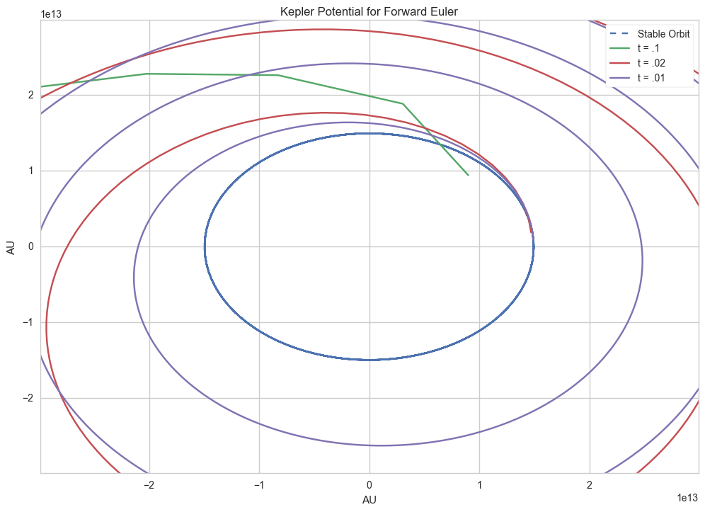
…Something went wrong. The forward Euler method is telling us that the Earth's orbit should spin out of control within 10 years, even less if we're taking bigger timesteps!

So why is our Earth in the forward Euler problem spinning into oblivion? We'll have to introduce the concept of symplectic integrators. Basically what it means is that a symplectic system is one that is time reversible, that is, the system itself preserves it's transformations and is time reversible. The reason why the forward Euler method causes the Earth to spin into the outer reaches of the solar system is that the method doesn't preserve the phase of the system, so the tiny phase errors within each timestep add up until our Earth spirals out of orbit. How do we solve this problem? A tiny modification to the Euler method allows us to preserve the phase:

\(\begin{gathered} v^{n+1}_p = v^{n}_p + a(x^{n}_p)\Delta t \end{gathered}\)

\(\begin{gathered} x^{n+1}_p = x^{n}_p + v^{n+1}_p\Delta t \end{gathered}\)

This doesn't look all that different, except that we're now using the velocity in the next timestep to calculate the next dimension. With this, the phase errors are preserved, and we get a much more reasonable orbit. So we'll write some code to fix that as well:

def modEuler(x, v, a):
    """Modified Euler method"""
    tempX, tempA = getAccel(x, a)
    #wonky, but quick and dirty array multiplication hack
    v = map(sum, zip(v, [i*dt for i in tempA]))
    x = map(sum, zip(tempX, [i *dt for i in v]))
    return (x, v)

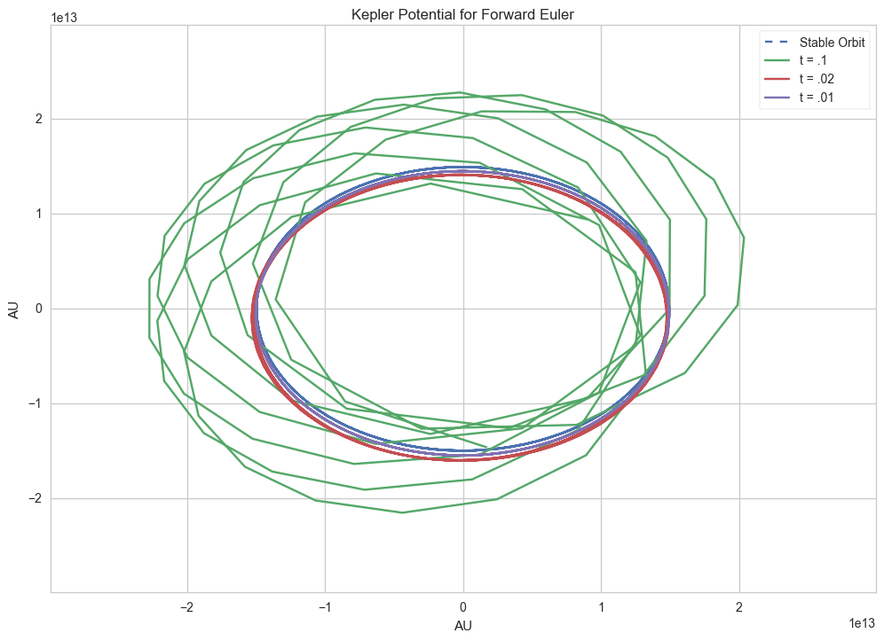
This is much closer to what we want, but there's still noticeable phase errors on the simulation. The errors are caused by the inherent linear-ness of the Euler methods, we're getting pretty close to it, but we need to go an order higher to get more accurate simulations, which is what I'll talk about at another time.